
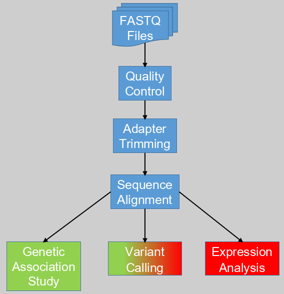
Next Generation Sequencing (NGS) data has slowly become the standard in bioinformatics, replacing PCR and microarray expression data. Though all three hold genetic information, NGS data is unique in that it directly gives the genetic sequences of a sample. Usually these sequences are stored in FASTQ formatted files. To analyze these files into something useful we develop software/computational pipelines.
A common first step in a pipeline is a quality control (QC) step with a tool such as FastQC. This is to ensure that the input, the FASTQ files are good. As they say, garbage in will only give garbage out. Thus it is important to measure the quality of the data. If you want to improve the pipeline further, you could implement a switch stopping the pipeline if the quality of the data is not high enough. Otherwise you can flag the data after it has been analyzed.
Once you know the quality of the input data it is time to prepare it for use. Almost all NGS data comes from Illumina sequencers, which uses specific short sequences bound to the actual sequences from the sample. These short sequences are called adapters and should be removed before further processing. The tools Cutadapt and Trimmomatic are commonly used for this purpose. Both tools can also be used for sequence trimming. This will remove nucleotide bases from the beginning and end of the sequence that are below par, though this will require some fine-tuning. It can be useful to look at quality of the data again at this point.
When you know that the data is prepped and ready we can go on the next step. With this step we align the sample sequences to a reference. This is achieved using aligner programs such as STAR, Bowtie2, and BWA. Each uses the reference as a template to match the sample sequences against to correctly place them to their corresponding genes (and other genetic locations). The reference is the entire genome that is comparable to the sample. So if you have human sample, use a human reference. It is recommended to use the latest reference available.
After creating the alignment, the follow-up steps will depend on the goal you want to achieve and the kind of NGS data you have. NGS data can largely be divided into DNA and RNA sequenced samples. With RNA sequenced data you measure the transcriptome, thus the activation of genes at a specific moment in time. DNA sequenced data on the other hand is more stable over time and describes the entire genetic landscape better.
The difference between DNA and RNA data can limit the kind of analysis you are able to perform. Each analysis has multiple steps that deserves its own blog post. So in short; An expression analysis can give us the genes that are activated, and by reverse inference thus also the ones that are deactivated. Of course this is limited to RNA data. A genetic association study on the other hand requires the stable DNA of many samples to find structural differences in the genome between populations. Variant calling, to uncover structural differences of one sample against a reference, can be done with both DNA and RNA data. Though DNA data usually gives higher quality results.
Depending on the data you have and the goals you want to achieve it will be necessary to adjust and refine the pipeline. My advise would be ITERATE. Start with the commands in the shell and fine-tune them to your liking. Iterate on the code and put it in a script to automate it, this can be any kind of script though shell scripts are advised. Further iterate by searching for processes that could be run in parallel or on multiple cores to make maximum use of the available hardware. It can be useful to use workflow software such as Snakemake or NextFlow at this point. Hopefully this post gives some guidance and helpful tips to start developing your NGS analysis pipeline.